Ross Driedger

Software Developer

London, Ontario, Canada
ross (at) earz (dot) ca

Pathfinding

Pathfinding is a very important part of video games. Non player or AI characters must give the impression of moving is a reasonable manner through their spaces. Consider the ghosts in the classic game Pacman: during most play, they tend to gravitate to Pacman, giving the player the challenge of avoiding them. The logic of the ghosts calculates a reasonable path to Pacman.

The two most commonly used algorithms are related: Dijkstra's Algorithm and A*. Both keep a list of 'open nodes' as possible paths to the goal. As soon as a path is found to be non-optimal or futile, it is placed on a lost of closed paths. This prevents the algorithm from searching where the solution cannot possibly be.

Dijkstra's Algorithm starts by finding the cheapest path that is unexplored. As soon as it discovers it it blind or that there is a cheaper path, it disregards it.

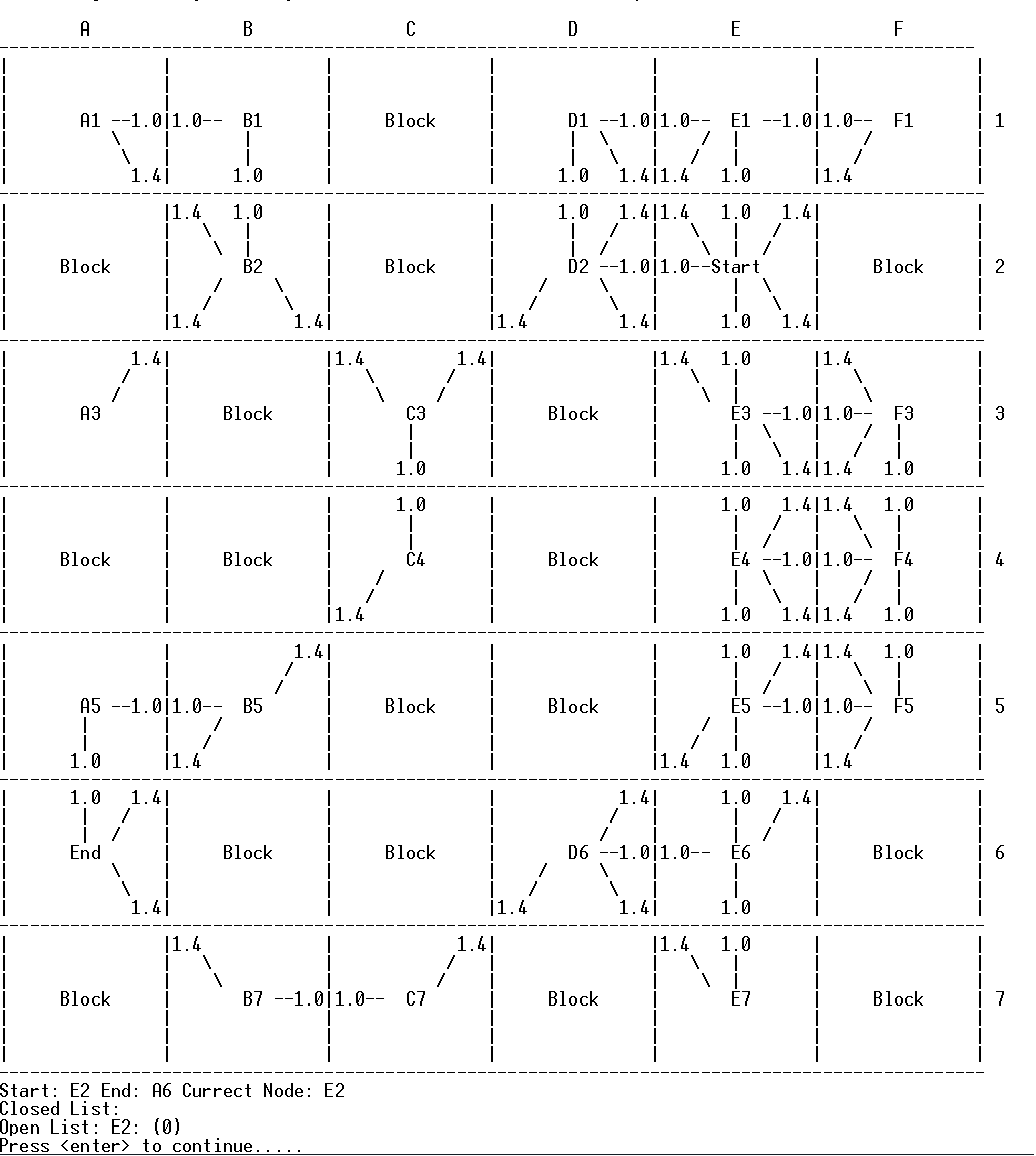
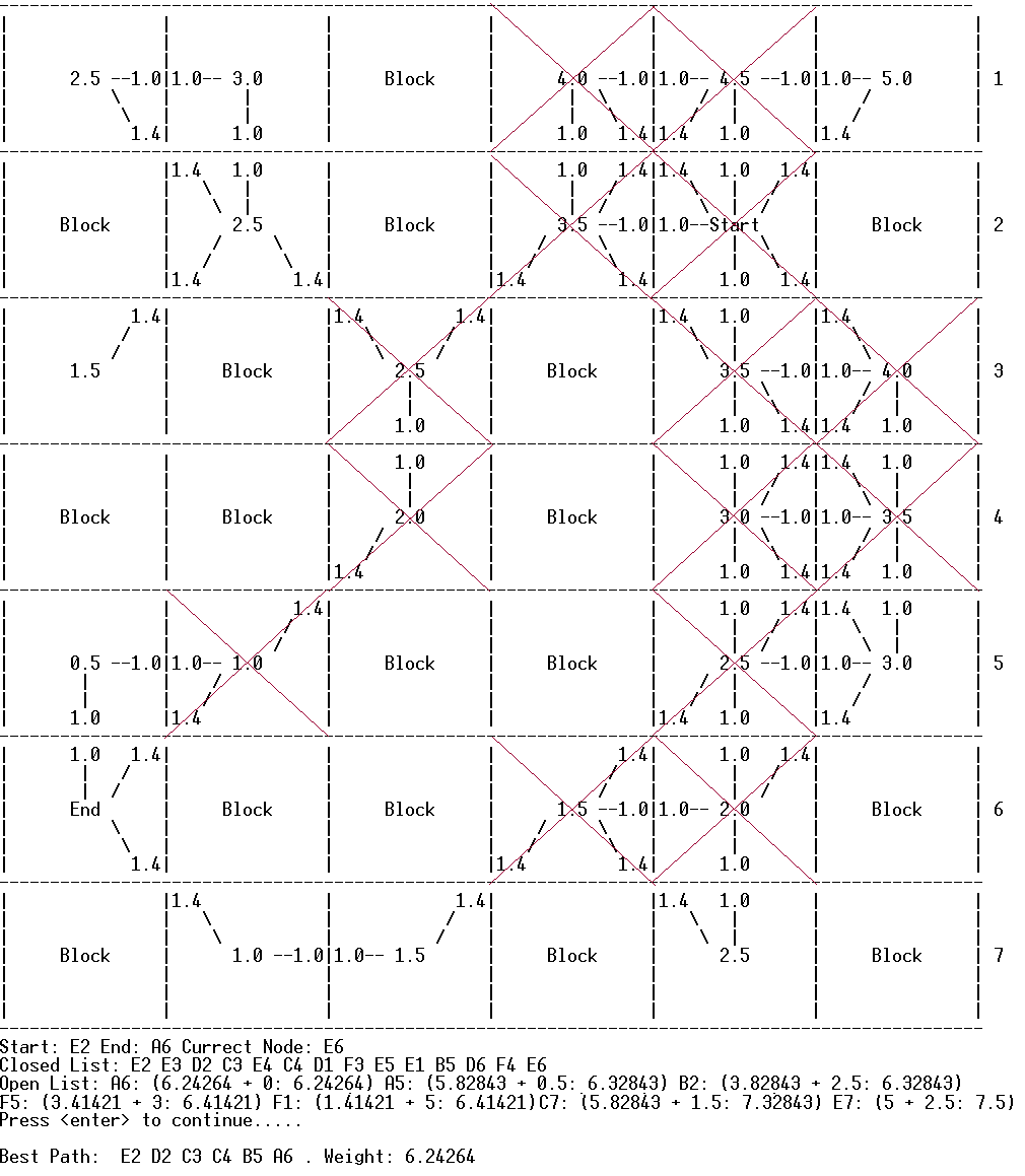
In this example, the path starts on square E2 and it must find the cheapest path to A6. Each move from square to square comes with a cost which is the number between the cells. In this example program, a grid is randomly generated, with some paths blocked and each move from one cell to another with a cost value.

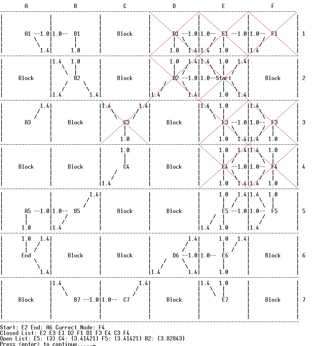
The cells on the closed list (marked in red on the diagram but does not shown in the program) show the progress of the algorithm as it works its way to the end cell.

Eventually the algorithm finds the optimum path from the start to end by finding the combination cheapest moves from cell to cell. In this screen shot the best path is indicated.

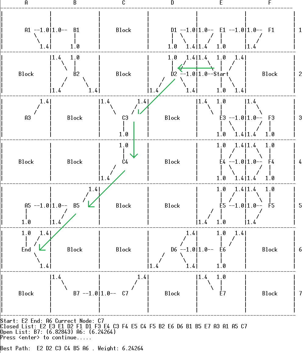
In this example you will notice that the closed list ends at twenty-three entries: only two cells were not visited in the pathfinding. This inefficiency is because Dijkstra's algorithm does not supply a clue as to whether a choice of cell is working toward or away from the end cell.

The A* algorithm (pronounced 'A-Star') adds a value to each cell called a heuristic. The heuristic offers an indication of whether the cell is more or less likely to be better or worse than another choice. In this case we use what is called the Manhattan Distance from the end cell to determine if a particular path is leading the algorithm in an optimal direction. The Manhattan distance is calculated as the sum of the vertical and horizontal cells to the end cell, divided by 2. In this case, the number of cells visited to find the optimal path was reduced to fourteen.

Choosing a heuristic can be a delicate adjustment. In a grid that has consistent path costs, a strong heuristic can find the optimal path much quicker in A* than in Dijkstra, but if the costs vary widely, a strong heuristic can lead to inefficiencies.

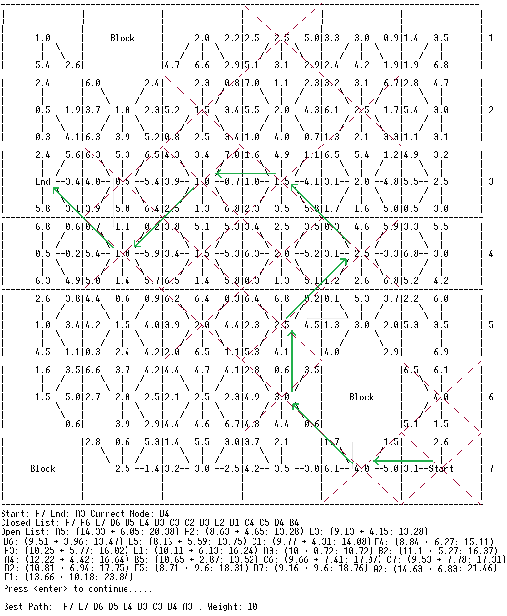
Here is a more varied example. Using Dijkstra's algorithm, the pathfinding visits 26 cells before it finds the optimal path. The green arrows show the best route and the visited cells are crossed out in red:

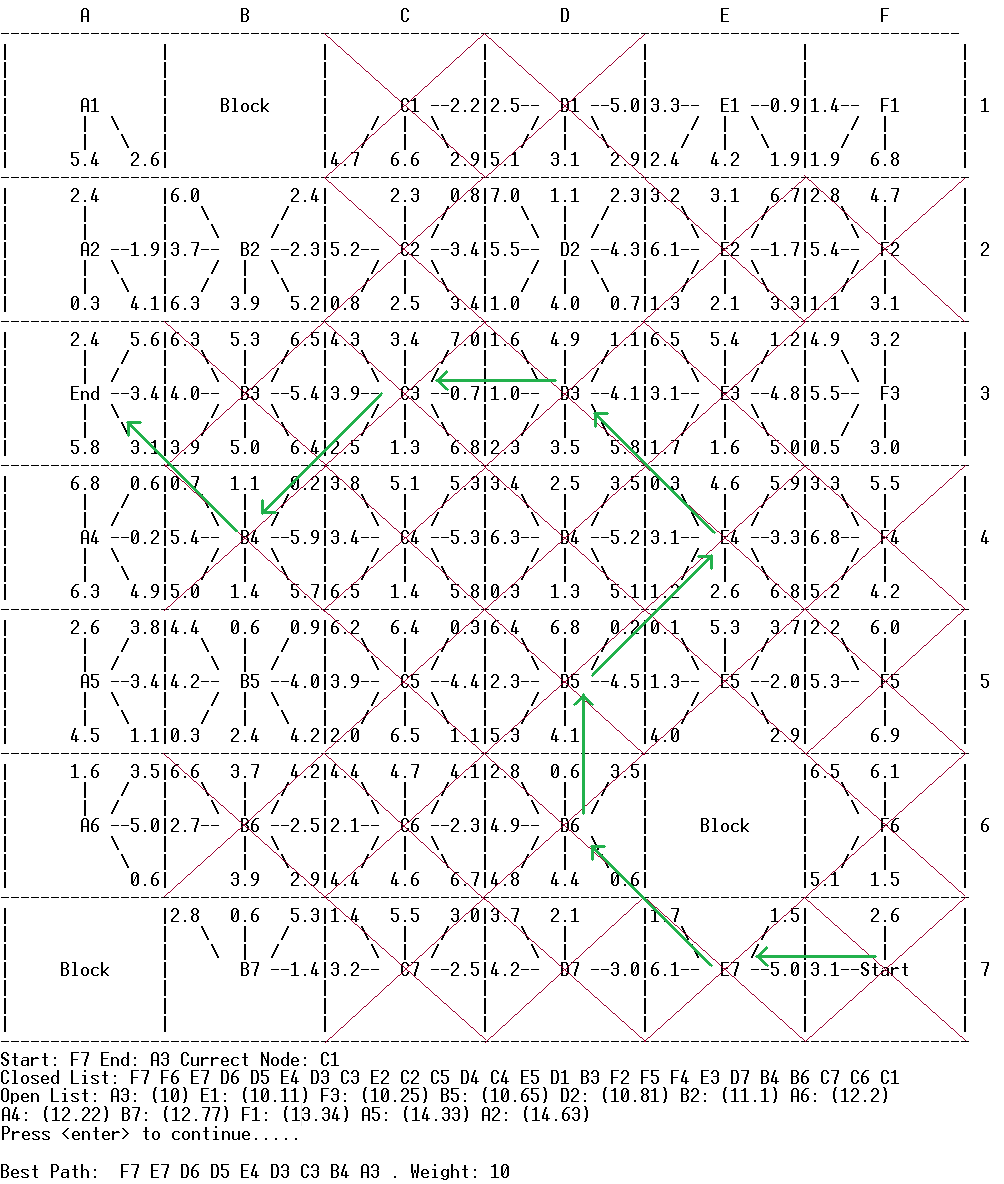
Using A*, many of the cells that lead away from the end are eliminated from the search. They are saved for possible evaluation later but the heuristic pushes the search in the correct direction. Only 16 cells are visited to find the same path as we found with Dijkstra.